Oscillator with odd nonlinearities

MMS example of an oscillator with odd (cubic, quintic and septic) nonlinearities subject to a direct harmonic forcing.

System description

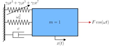
Illustration of a forced nonlinear oscillator with odd nonlinearities of degree 3, 5 and 7.

The system’s equation is

\[\ddot{x} + c \dot{x} + \omega_0^2 x + \gamma_3 x^3 + \gamma_5 x^5 + \gamma_7 x^7 = F \cos(\omega t),\]

where

• \(x\) is the oscillator’s coordinate,

• \(t\) is the time,

• \(\dot{(\bullet)} = \mathrm{d}(\bullet)/\mathrm{d}t\) is a time derivative,

• \(c\) is the linear viscous damping coefficient,

• \(\omega_0\) is the oscillator’s natural frequency,

• \(\gamma_3,\; \gamma_5, \; \gamma_7\) are the nonlinear coefficients,

• \(F\) is the forcing amplitude,

• \(\omega\) is the forcing frequency.

A direct response is sought so the frequency (either backbone curve frequency or forcing frequency) is close from the oscillator’s, such that

\[\omega = \omega_0 + \epsilon \sigma,\]

where

• \(\epsilon\) is a small parameter involved in the MMS,

• \(\sigma\) is the detuning wrt the reference frequency \(\omega_0\).

The parameters are then scaled to indicate how weak they are:

• \(c = \epsilon^{N_e} \tilde{c}\) indicates that damping is weak (of order \(N_e\)),

• \(F = \epsilon^{N_e} \tilde{F}\) indicates that forcing is weak (of order \(N_e\)),

• \(\gamma_i = \epsilon \tilde{\gamma}_i, \; i=3, 5, 7\) indicates that nonlinearities are weak (of order 1).

Note that \(N_e\) is the order up to which the solutions are sought and the time scales are constructed. It is therefore chosen here to scale the damping and forcing at maximum order.

Code description

The script below allows to

• Construct the dynamical system

• Apply the MMS to the system up to order \(N_e=3\)

• Evaluate the MMS results at steady state

• Compute the forced response and the backbone curve

• Evaluate the stability of the computed forced solution.

• Evaluate the steady-state results for given numerical values of the parameters and plot the results.

# -*- coding: utf-8 -*-

#%% Imports and initialisation
from sympy import symbols, Function
from sympy.physics.vector.printing import init_vprinting, vlatex
init_vprinting(use_latex=True, forecolor='White') # Initialise latex printing 
from oscilate import MMS

# Parameters and variables
omega0, F, c = symbols(r'\omega_0, F, c', real=True,positive=True)
gamma3       = symbols(r'\gamma_3',real=True)
gamma5       = symbols(r'\gamma_5',real=True)
gamma7       = symbols(r'\gamma_7',real=True)
t            = symbols('t')
x            = Function(r'x', real=True)(t)

# Dynamical system
Eq = x.diff(t,2) + omega0**2*x + gamma3*x**3 + gamma5*x**5 + gamma7*x**7 + c*x.diff(t)
dyn = MMS.Dynamical_system(t, x, Eq, omega0, F=F)

# Initialisation of the MMS sytem
eps            = symbols(r"\epsilon", real=True, positive=True) # Small parameter epsilon
Ne             = 3      # Order of the expansions
omega_ref      = omega0 # Reference frequency
ratio_omegaMMS = 1      # Look for responses around the reference frequency (Default behaviour)

param_to_scale = (gamma3, gamma5, gamma7, F , c )
scaling        = (1     , 1     , 1     , Ne, Ne)
param_scaled, sub_scaling = MMS.scale_parameters(param_to_scale, scaling, eps)

mms = MMS.Multiple_scales_oscillator(dyn, eps, Ne, omega_ref, sub_scaling)

# Application of the MMS
mms.apply_MMS(orders_polar=0)

# Evaluation at steady state
ss = MMS.Steady_state(mms)

# Solve the evolution equations for a given dof
solve_dof = 0 # dof to solve for
ss.solve_forced(solve_dof=solve_dof)
ss.solve_bbc(solve_dof=solve_dof, c=param_scaled[-1])

# Stability analysis
ss.stability_analysis_forced(coord="polar", eigenvalues=True, bifurcation_curves=True)

# Plot the steady state results
# -----------------------------

# Set parameters' numerical values
import numpy as np
param = [(omega0, 1),
         (c, 1e-2),
         (gamma3, 0.2),
         (gamma5, -0.3),
         (gamma7, 0.12),
         (ss.coord.a[0], np.linspace(1e-10, 2, 1000))]

# Frequency response
param_FRC = param + [(dyn.forcing.F, 1.4e-2)]
BBC = MMS.visualisation.Backbone_curve(mms, ss, dyn, param_FRC)
FRC = MMS.visualisation.Frequency_response_curve(mms, ss, dyn, param_FRC)
FRC.plot(ss=ss, bbc=BBC)

# Amplitude response
param_ARC = param + [(mms.omega, 1.02)]
ARC = MMS.visualisation.Amplitude_response_curve(mms, ss, dyn, param_ARC)
figs_ARC = ARC.plot(ss=ss)
[fig.get_axes()[0].set_xlim(0, 0.04) for fig in figs_ARC]

# %%

Plot outputs

The plot outputs shown below are generated from the code above.

Frequency response curve

The two figures below display the amplitude and phase responses (blue) of the \(1^{\text{st}}\) harmonic of the nonlinear oscillator as a function of the excitation frequency and the associated bifurcation curves (red), delimiting unstable from stable zones. The backbone curve is shown in grey and the linear frequency in black.

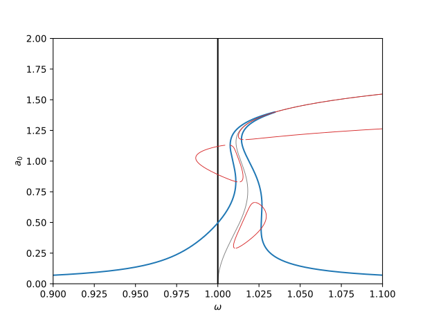
Frequency response curve of the nonlinear oscillator (amplitude).

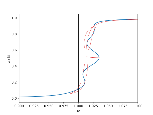
Frequency response curve of the nonlinear oscillator (phase).

Amplitude response curve

The two figures below display the amplitude and phase responses (blue) of the \(1^{\text{st}}\) harmonic of the Duffing oscillator as a function of the excitation amplitude.

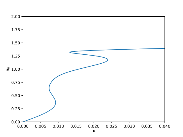
Amplitude response curve of the nonlinear oscillator (amplitude).

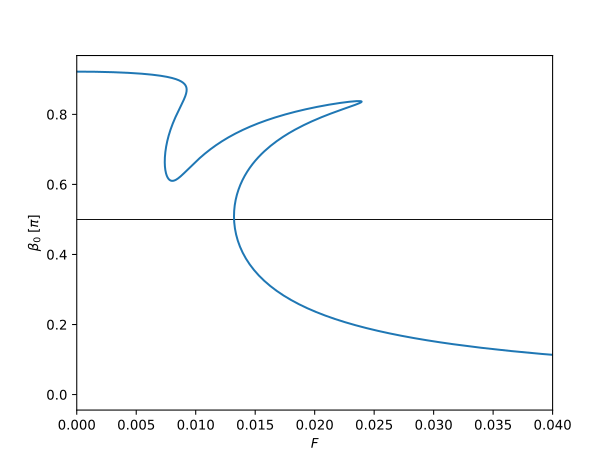
Amplitude-response curve of the nonlinear oscillator (phase).